Visualization of electron density maps from Jana2000 vith OpenDx
OpenDx is an open source version of IBM's Visualization Data Explorer. It can be downloaded from
www.opendx.org. Plotting of isosurfaces is
just a small subset of the OpenDx possibilities. In this document we provide a quick
guide to plotting Contour output. Advanced usage requires reading of OpenDx documentation.
Installation of OpenDx
Currently we have experience only with the version for Windows98. We downloaded opendx-4.1.3-2-WIN32-setup.zip
from the OpenDx page. After decompression we ran the setup program in a standard way known to Windows users.
OpenDx has been originally developed for Unix platforms and in Windows it needs a running X11 emulation program.
We have been using eXceed.
Problems:
Sometimes the program stopped working with messages like "Server connection broken" or
"Could not connect to dxexec". Solution: restart of OpenDx.
Exceed worked correctly except problems with keyboard buttons like arrows, Home, End etc. These
buttons did not work in the graphics interface but they could be replaced with mouse operations.
Preparation of data with Jana2000
Only maps generated in orthogonal axes can be saved in the stf file format without deformation.
All crystal systems
Calculate Fourier map in an independent volume

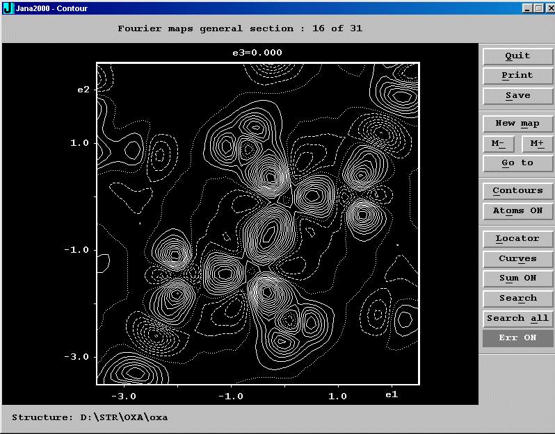
In Contour choose "General section"
Define a section of non-zero width. An interpolation step about 0.1A is sufficient for
smooth contours.
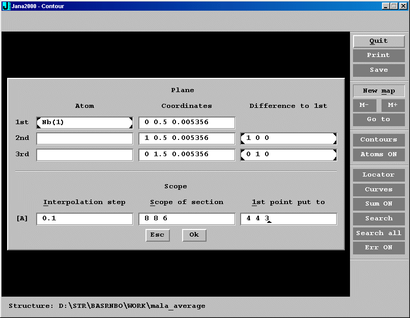
Save all sections in the stf format

Another possibility for orthogonal, tetragonal and cubic systems
Calculate Fourier map in a user-defined volume. In the given example "Step" is in
fractional units.

In Contour choose "Fourier map(s) from m81 file"
Save all sections in the stf format
Starting OpenDx
We assume the program has been installed in default location c:\opendx. The main program menu is
started by c:\opendx\bin\Menu.bat. Don't forget that an X11 emulation must be running in this
time.
Preliminary work
OpenDx provides a lot of functions that can be used for creation of OpenDx programs. Such a program
is necessary also for plotting of isosurfaces. Fortunately it can be created like a copy of
a demo sample. Another necessary file contains data description. Both files - the program and the data description -
can be created once for all and then only edited with respect to plotted data.
In the following two paragraphs we shall create the program file "program.net" and the data description file
"data.general". The extensions ".net" and ".general" are mandatory, the basic names are
arbitrary.
Creation of program file "program.net"
Choose "Edit visual programs"
Open file c:/opendx/samples/tutorial/Isosurface3D.net. It will start the "Visual program editor".
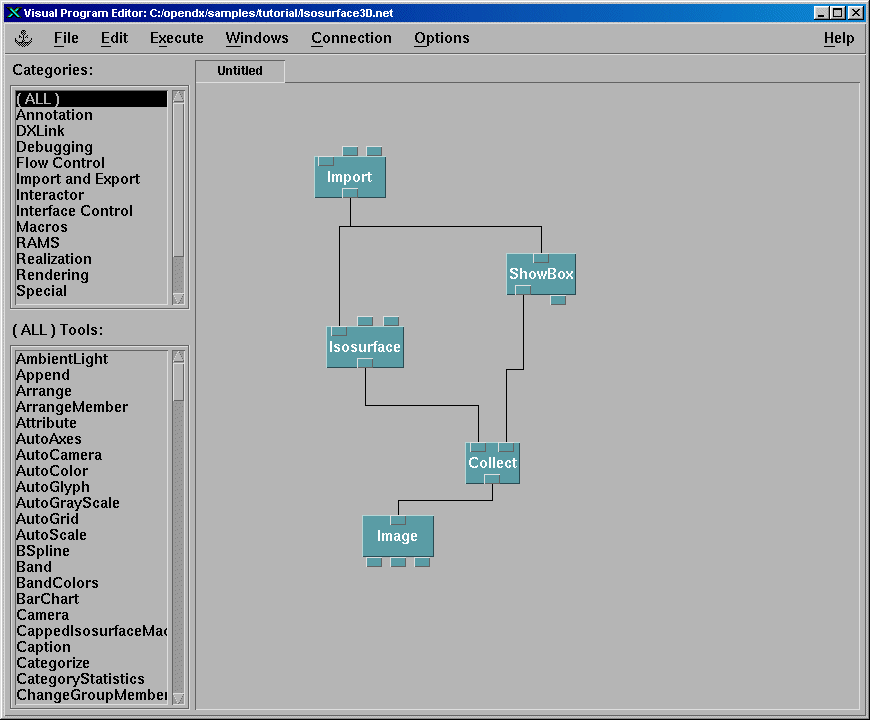
Double-click "Import". It will open the Import dialogue. Check "Name" checkbox and replace
the string "cloudwater.dx" with c:/opendx/data.general. This is the name of the data description file
that we shall create later. The quotes " can be omited. Note that we are using unix-like slash /
though the system is Windows.

Close the Import dialogue and choose "File" and "Save As".
Save the program with name c:/opendx/program.net
Close the window "Edit visual programs"
Creation of data description file "data.general"
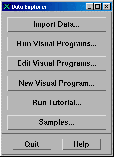
Choose "Import data". It will open the "Data Prompter" dialogue. Select
"Grid or Scattered file".
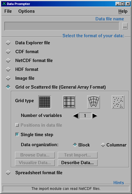
Press "Describe data". It will open the second "Data prompter" box.
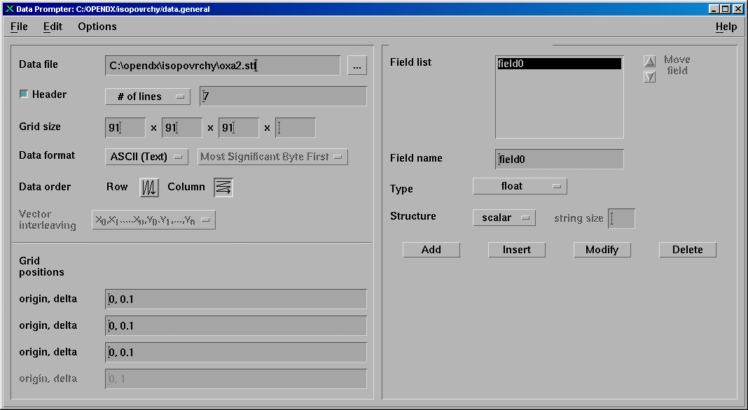
In the "Data file" textbox fill in the pathname of your stf file
In the "Header" choose "# of lines" and type 7. This is the stf header that should be
skipped by OpenDx.
Type the grid size according to the stf file header
Select "Data order" = "Column"
In the Grid positions "origin" is 0 and "delta" is the interpolation step
used for calculation of General section by Contour program (usually 0.1).
Choose "File" and "Save as" and save the data description in c:/opendx/data.general
Close both windows of "Data prompter"
Close OpenDx by "Quit" button in the mani menu of OpenDx. If you want continue with the
next paragraph of this recipe close OpenDx and start it again in order to get
the standard behaviour.
Plotting of isosurfaces
In this part we assume that both the program file (c:/opendx/program.net) and the data
description file (c:/opendx/data.general) have been already created.
Start the main program menu by c:\opendx\bin\Menu.bat.
Choose "Import data" in the main menu of OpenDx. It will open the "Data prompter" window.
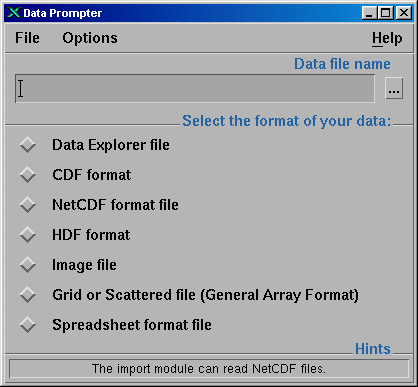
In the "Data file name" textbox type the fullname of the data description file, i.e.
c:/opendx/data.general and press Enter. This will select "Grid or scattered file" checkbox
and open the second window of the Data prompter.
Edit definitions according to your stf file. Then save the description file
by choosing "File" and "Save".
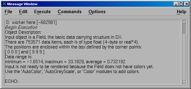
In the first window of the Data prompter press "Test import" button. This will test
whether your stf file is readable. The testing may take a while. The test results are
displayed in the "Message window".
Close all windows except the main menu
In the main menu choose "Run visual programs". In the "File selection" dialogue
find c:/opendx/program.net. Press OK. After some time dependent on the size of the map
the "Image" window will appear in the screen. After pressing Ctrl-F the image of electron
density will appear in the "Image" window.

In the "Image" window choose "Windows" and "Open visual program editor". This will
open the Visual program editor.
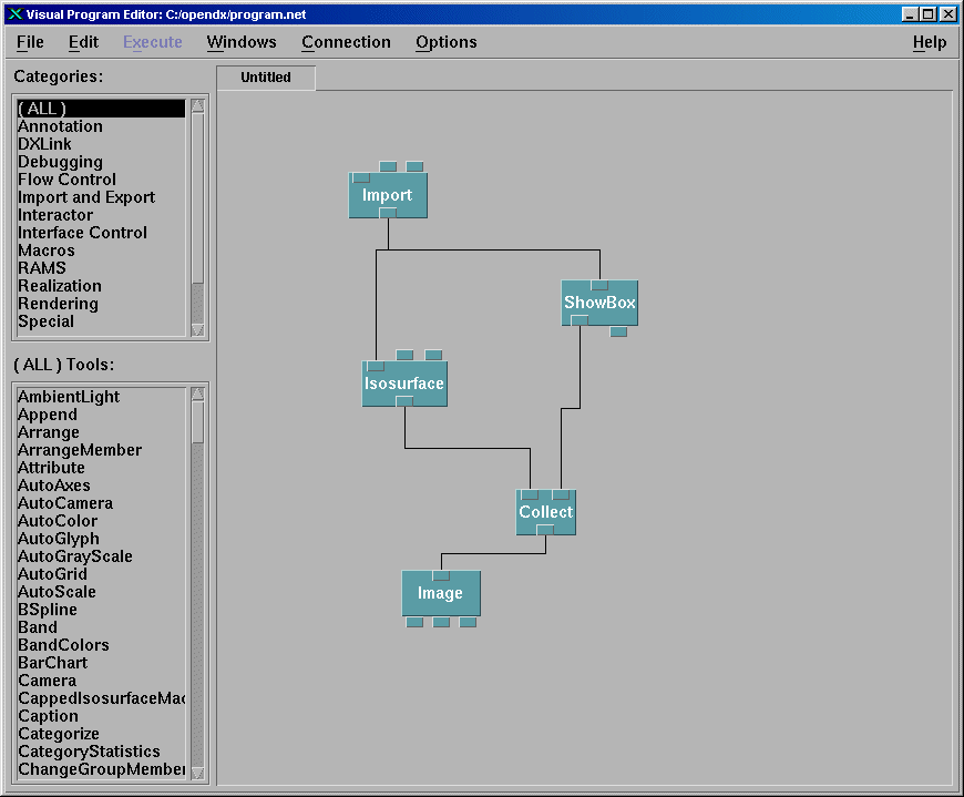
Double-click "Isosurface". This will open the "Isosurface" dialogue.
Select the "Value" checkbox and type the electron density limit. The value depends on the
plotted map and can be estimated with "Locator" of the Contour program.

Press "Apply" or "OK" button. The image will be automatically redrawn. Close the
"Visual program editor" window.

The image should be in the same orientation like in the Contour plot. If you don't see
what you have expected a possible reason could be that OpenDx remembers the last picture.
Restart of OpenDx solves it (though we believe there is also some more elegant
solution).
In the "Image" window choose "Options" and "View control". Then the image
can be rotated or scaled. The last figure shows the image after rescaling.

The image can be saved in various formats by choosing "File" and "Save image"
Note
We are not experienced users of OpenDx and we cannot guarantee this recipe shows the
best way of displaying Jana electron density maps.